
My last post about pushing over 10 000 square kilometres of lidar coverage as Entwine Point Tiles was driven by the arrival of a whole bunch of data over Kosciuzsko National Park / Ngarigo country. This was intended for extending a work-in-progress avalanche risk map to include vegetation structure, and also cover more area. Her’s some initial work here, mixing slope-at-risk-of-avalanche (red) with terrain convexity (blue). It is far from done, we’ll discuss that another time.

…but then, things got out of hand.
Being a crazy point cloud guy, I figured I’d turn them into an Entwine Point Tile index and republish them. But what could I add? For just points, Geoscience Australia does a great job of providing the data (thats how I got them). I figured colour – sticking by my principles about data explorability, and also testing a brand new capability in PDAL – making height above ground (normalised height) using locally-triangulated meshes.
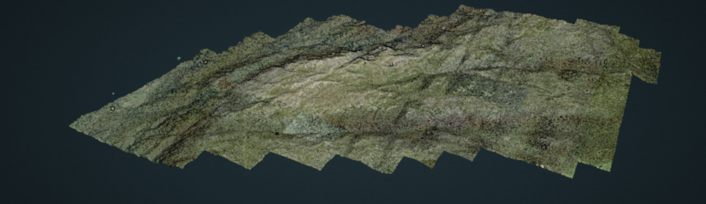
Here’s what turned up. When funding allows, these data will be fully interactively explorable again.
To make this happen I needed to:
- find an imagery source
- clip bits of imagery to match my las tiles
- construct some glue to process a few hundred las tiles
Lets start at part 1 – finding imagery.
Fetching and clipping WMTS imagery with GDAL
The first issue with the plan was that I didn’t have a local copy of imagery to colour my points with using recipes I’d made before. However – New South Wales (NSW) Government offers an excellent web map tiling service of ‘latest available’ imagery, and I found GDAL’s WMTS driver. This took some getting my head around – with initial attempts pretty much trying to download the entire NSW imagery dataset into one raster at all zoom levels.
Here’s the web map tile server GetCapabilities URL:
https://maps.six.nsw.gov.au/arcgis/rest/services/public/NSW_Imagery/MapServer/WMTS/1.0.0/WMTSCapabilities.xmlDon’t go too mad reading the XML – we let GDAL do a lot of the heavy lifting for us! However, we do need to look for the image layer identifier:
<heaps_of_xml>
<Layer>
<ows:Title>public_NSW_Imagery</ows:Title>
<ows:Identifier>public_NSW_Imagery</ows:Identifier>
<heaps_more_xml>
…which we pass to GDAL along with the GetCapabilities URL to generate a create a configuration file – like this:
gdal_translate “WMTS:https://maps.six.nsw.gov.au/arcgis/rest/services/public/NSW_Imagery/MapServer/WMTS/1.0.0/WMTSCapabilities.xml,layer=public_NSW_Imagery” wmts-template.xml -of WMTSThe resulting XML output in wmts-template.xml looks something like this:
<GDAL_WMTS>
  <GetCapabilitiesUrl>https://maps.six.nsw.gov.au/arcgis/rest/services/public/NSW_Imagery/MapServer/WMTS/1.0.0/WMTSCapabilities.xml</GetCapabilitiesUrl>
  <Layer>public_NSW_Imagery</Layer>
  <Style>default</Style>
  <TileMatrixSet>default028mm</TileMatrixSet>
  <TileMatrix>18</TileMatrix>
  <DataWindow>
    <UpperLeftX>xmin</UpperLeftX>
    <UpperLeftY>ymax</UpperLeftY>
    <LowerRightX>xmax</LowerRightX>
    <LowerRightY>ymin</LowerRightY>
  </DataWindow>
  <BandsCount>4</BandsCount>
  <Cache />
  <UnsafeSSL>true</UnsafeSSL>
  <ZeroBlockHttpCodes>204,404</ZeroBlockHttpCodes>
  <ZeroBlockOnServerException>true</ZeroBlockOnServerException>
</GDAL_WMTS>
…I say something – because I’ve added the tilematrix field and swapped the coordinates for placeholder strings. The gdal_translate command issued above fills these values with the full extent of the WMTS tileset!
tilematrix is more or less ‘zoom level’. Without specifying this, GDALs WMTS driver will think you want all the zoom levels. I’d already inspected my lidar dump, and zoom level 18 (corresponding to ~0.5cm/pixel) was plenty for this job. This is a little trial and error – try grabbing a small chunk of imagery to test your ideas about what the zoom level means, before hammering away at multiple requests…
Geobash!
Now that we have our images we need glue. I chose bash programming! It’s built into linux, I kind of know how to do stuff in it, and find it easier than building in Python or whatever else for generating quick proof-of-concept work. It’s also really recyclable.
Geobash is like regular bash – the bourne again shell – used to drive geo-things. In this case processing for a couple hundred lidar tiles with GDAL and PDAL. And I am not the only geobash afficionado on the planet – an excellent example from XYCarto helped inspire me to write this one up.
While bash is really quirky, and not well loved by all, it has some really neat capabilities. One of those is being able to string together existing programmes to do complex task (aka pipelines) – which also flows backwards, to being able to test components easily. There are a lot of tutorials around using bash to string things together – searching for the thing you need to do is the best way to get into using it.
Because I find programming in anything is hard and quirky, I write all of this stuff with a terminal, text editor and search window open at all times – sometimes every line of code has a ‘how do I do…’ search behind it…
Setting up for some geobash
All our components are now ready. LAS tiles, a template for WMTS imagery, GDAL and PDAL, and bash. The output I wanted was colourised points, with height above ground (relative height) precomputed. What I needed to do next was for each las tile:
- find its bounding region
- convert las tile bounds to WMTS coordinates
- grab a chunk of imagery
- warp imagery to las tile coordinates
- use PDAL to colourise points from imagery
- use PDAL to compute height above ground
- write out a laszip compressed LAS 1.4 tile with colours and height above ground as an extra dimension
A shell script to do all of that is given below. Hopefully the comments in the code tell you everything you need to know. Note – I tested this extensively as a single-las-tile script before wrapping a for loop around it. Because its 2020 I really should be showing you how to run all your CPUs hot and parallelise it all. That might turn up later.
In linux/unix shells, the pipe operator | is how things are strung together. It means ‘take the output of the command before the vertical pipe and send it to the command after the pipe’ – so, where you see cat pdalinfotemp.json | jq that means ‘use the program cat to spit out the contents of pdaltempinfo.json and give those straight to the jq JSON interpreter to do things with.
Where you see syntax like thing=$(cat pdalinfotemp.json), we’re assigning the variable thing the output of the operation inside the brackets – which can be fairly complex in itself. Where there are curly brace assignments like thing=${coordsarray[0]}, we’re looking into a bash array to grab an element. And finally, > is a redirection in bash.
I hope thats enough bash weirdness to get into this script…
#!/bin/bash
#shabang! it’s geobash
# this script takes one parameter - a directory full of las tiles.
# it expects two output directories to exist:
# ./imagechunks (where imagery captured from WMTS are dumped)
# ./laz-colour-hag (where output laz files are written)
#
# so the directory structure looks like:
# /path-to/wmts-lidar-colouriser.sh
# /path-to/input-lastiles-are-here
# /path-to/imagechunks
# /path-to/laz-colour-hag
#
# run like:
# > bash wmts-lidar-colouriser.sh ./input-lastiles-are-here
# (yes, be sure to say bash)
#################################################

#set up a for loop, read lasfiles in the input folder
for f in $1/*.las
    do
        lazfile=$f
        #print the file name as a check
        #echo $f
        # remove a template vrt from imagechunks
        if [ -f ./imagechunks/wmts-chunk-tf.vrt ]; then
            rm ./imagechunks/wmts-chunk-tf.vrt
        fi

        #drop directory tree and extension from the las file name
        thefile=$(basename $lazfile .las)

        #print it’s name - as a visual check
        echo $thefile

        # collect a pdal boundingbox and xmin/xmax/ymin/ymax
        # and save the results in pdalinfotemp.json
        # note that the bbox limits then have 50m added, to ensure that
        # the raster fully covers all lidar points
        # pdalinfotemp.json is over-written for each tile.

        echo "getting las file extents"
        pdal info --summary $f > pdalinfotemp.json

        # read the JSON we just made and extract stuff we want.
        # we also add a 50m buffer to each bounding box corner using
        # the bash calculator (bc)
        minx=$(cat pdalinfotemp.json | jq '.summary.bounds.minx')
        minxb=$(echo $minx-50 | bc)
        maxx=$(cat pdalinfotemp.json | jq '.summary.bounds.maxx')
        maxxb=$(echo $maxx+50 | bc)
        miny=$(cat pdalinfotemp.json | jq '.summary.bounds.miny')
        minyb=$(echo $miny-50 | bc)
        maxy=$(cat pdalinfotemp.json | jq '.summary.bounds.maxy')
        maxyb=$(echo $maxy+50 | bc)

        # next, we fill a variable wmtscoords with the output of an
        # operation reprojecting our las corner coordinates in
        # MGA/GDA94 to wmts coords in web mercator, using cs2cs. Note
        # the proj strings are not dynamic, you have to reconfigure
        # the transformation here if your data are not in EPSG:28355

        # quick bash note - the <<EOF..EOF part means ‘feed text between the
        # matching EOF pairs into the command we’ve just defined’.

        wmtscoords=$(cs2cs -f "%.6f" +proj=utm +zone=55 +south +ellps=GRS80 \
            +towgs84=0,0,0,0,0,0,0 +units=m +no_defs +to +proj=merc +a=6378137 +b=6378137 \
            +lat_ts=0.0 +lon_0=0.0 +x_0=0.0 +y_0=0 +k=1.0 +units=m +nadgrids=@null +wktext \
            +no_defs <<EOF
$minxb $minyb
$maxxb $maxyb
EOF
        )
        #spew out coords to check if needed
        #echo $wmtscoords

        #replace spaces with commas using sed - because I couldn’t figure out
        #spaces for the next part...
        wmtscoords=$(echo $wmtscoords | sed 's/ /,/g')

        #…which is loading a bash array with coordinates
        # this seemed easier than a regular expression to extract
        # bits of the $wmtscoords string
        # the <<< is a redirection which is bash specific
        IFS="," read -ra coordsarray <<< "$wmtscoords"

        #assign min/max coords for wmts image capture from the array
        xmin=${coordsarray[0]}
        ymin=${coordsarray[1]}
        xmax=${coordsarray[3]}
        ymax=${coordsarray[4]}

        # $bbox is never used, it was for printing to the terminal I think..
        # retained here because it demonstrates assembling a comma delimited string
        # from a bash array.
        bbox=$(echo ${coordsarray[0]},${coordsarray[1]},${coordsarray[3]},${coordsarray[4]})

        # now some fun with sed! using the WMTS xml template we made,
        # spawn a temporary version with our las file bounds injected
        # where we had string placeholders. We’re using > in the first operation to say
        # replace a string in our template with a value, and write the result
        # to a new xml file.

        sed 's/xmin/'$xmin'/' nsw-wmts-template.xml > wmts-chunk.xml
        sed -i 's/ymin/'$ymin'/' wmts-chunk.xml
        sed -i 's/xmax/'$xmax'/' wmts-chunk.xml
        sed -i 's/ymax/'$ymax'/' wmts-chunk.xml

        # next, see if we already have this image chunk downloaded...
        echo "testing for existing image"
        if [ ! -f ./imagechunks/wmts-chunk-$xmin-$ymin-$xmax-$ymax.tiff ]; then
            # if not - use gdal translate to transform our
            # WMTS config into an honest-to-goodness geotiff

            echo "getting wmts"
            gdal_translate wmts-chunk.xml ./imagechunks/wmts-chunk-$xmin-$ymin-$xmax-$ymax.tiff
        fi

        # then, reproject the raster into lidar coordinates
        # and ouput a VRT
        echo "warping raster"
        gdalwarp -s_srs EPSG:3857 -t_srs EPSG:28355 -tr 0.5 0.5 -r lanczos ./imagechunks/wmts-chunk-$xmin-$ymin-$xmax-$ymax.tiff ./imagechunks/wmts-chunk-tf.vrt -of VRT

        #now that the raster wrangling is done, we get to points! yay!
        echo "colourising points"
        pdal pipeline ./pdal-pipelines/hag-colour-pipeline.json --readers.las.filename=$f --filters.colorization.raster=./imagechunks/wmts-chunk-tf.vrt --writers.las.filename=./las-colour-hag/$thefile.laz -v 8

        # and finally we close the loop.
        done
Running some geobash
Assuming we saved this script as ‘wmts-lidar-colouriser.sh’, it is run at the shell prompt using:
bash wmts-lidar-colouriser.sh ./path-to-lasfiles/It is not particularly clever in that it doesn’t create directories for temporary or intermediate or even output products for you, you need to create the directories imagechunks and las-colour-hag before you start.
For this script you must specify bash as the shell program to use – since it relies on a bash quirk to create the array of coordinates at line 78.
The attendant PDAL pipeline
In a way the geobash part is a long preamble to running a PDAL pipeline to compute height-above-ground and colourise points. This is the pipeline:
[
    "inputfile.laz",
    {
        "type":"filters.hag_delaunay",
        "count": 64,
        "allow_extrapolation": true
    },
    {
        "type":"filters.colorization",
        "raster": "raster"
    },
    {
        "type":"writers.las",
        "filename":"outfile.laz",
        "extra_dims": "all",
        "minor_version": 4,
        "dataformat_id": 7,
        "a_srs": "EPSG:28355+5711"
    }
]
…this is relatively straightforward: Ingest some points, compute height above ground ignoring noise, apply colour from a raster, and save the result in a modern LAS format. Our geobash wrapper provided input and output file names, and appropriate raster names as command line parameters to this pipeline
Recap
This story walks through getting some serious geospatial work done using a tool which comes with every *nix based computer – the shell terminal. We’ve used it to drive a series of open source geospatial libraries, pulling on open data sources, and deploying some pretty old tricks in the *nix book to move things around and glue it all together. We have:
- queried a pile of lidar files to find geospatial bounds
- collected aerial imagery tiles from a web map tile service using open standards
- reprojected string coordinates and raster data
- applied colour from raster data to lidar points
- computed normalised height for lidar
- written out modern compressed las tiles (LAS 1.4 data format 7 with extra dimensions)
The demonstration data for this covered 900 square kilometres. It took maybe a day and a bit to process, and could be a few times faster with not much modification to use inbuilt parallelisation tools (xargs, parallel). Given that the image tiles were all cached, the entire dataset has been reprocessed again to use more ground points when computing temporary surfaces for normalised heights.
This post seems pretty arduous – the point, really, is to show that if you have a shell prompt and a few key tools, you already have an incredible geospatial analysis system at hand! It is definitely worth spending a little time learning about it…
.
The sales pitch
Spatialised is a fully independent consulting business. Everything you see here is open for you to use and reuse, without ads. WordPress sets a few cookies for statistics aggregation, we use those to see how many visitors we got and how popular things are.
If you find the content here useful to your business or research or billion dollar startup idea, you can support production of ideas and open source geo-recipes via Paypal, hire me to do stuff; or hire me to talk about stuff.