
This is both a consumer grade RPAS (remotely piloted airborne system) write-up, and part 3 of the ‘open source point cloud infrastructure’ series (see part 1 and part 2) – looking at much smaller scale data produced by consumer (and other) RPAS systems using cameras.
The story starts with purchasing a tiny airplane to support a recent project for Synthesis Technologies.
After much internal debate I bought a Parrot Anafi. The selection process was an optimisation of cost, other people’s reviews of camera quality, and noise. The Anafi’s 180-degree gimbal was also an attractive feature, with some interesting future possibilities.
Here’s what it looks like:

One thing the Anafi lacks is collision avoidance – unlike it’s biggest competition (the DJI Mavic), it will run into stuff. This was a big decision being a relatively new RPAS pilot. And, of course, I learned the hard way during early flight testing. The camera gimbal on Anafi MK 1 was destroyed during a test flight under my patio eaves involving a 4 metre fall to brick (gimbal-first). However, the rest of the airframe survived intact – and an expensive lesson with an almost complete set of spare parts later, Anafi MK 2 is going strong with a number of missions under her belt now. I also bought a Ryze/DJI Tello (for the kids – really!) to gain flight time in tight spots with less risk.
A strong selling point of Anafi is it’s quietness – or at least it’s ‘less harsh noise’. I’ll let someone else demonstrate that for you here. It’s almost silent as soon as it’s 40 m or so away.
I’ve enjoyed that it is really easy to fly in manual mode, and takes instruction from Pix4D capture easily and intiutively. It’s behaviour on aborted missions is great – it hangs out awaiting instruction, and is easy to manually fly home. Using Parrot’s own flight planner is a bit more tedious – although offers much greater control over how imagery is collected using gimbal control at each shot, and also the ability to follow terrain (not automagically). I haven’t used it for data collection yet, preferring to use either Pix4D capture or fly manually.
And it packs up small. My entire data collection kit, minus ground control points, packs up into a repurposed climbing harness bag – the aircraft, a spare battery, controller, spare propellors, and a ground mat for launching (which is a repurposed tent footprint):

Data samples
Overhead flight / low oblique imagery
The reason for the existence of Anafi in my life was a need to simulate rapid data acquisition and processing using consumer-grade micro-aircraft. Conveniently, a new building was recently constructed in some forest nearby, away from roads and people – offering a great place to demonstrate some capability.
Firstly, here is a video overflight of the target structure:
…and here’s one result from a 6 minute flight, collecting 68 images, and using OpenDroneMap to process imagery into a dense point cloud:

This example was derived from a circular flight, where all images are taken looking inward at the target structure – without flying over it. As part of the exercise, I’ve just used the aircraft GPS and no ground control points (simulating no ground access). For this particular flight pattern, mismatch with a fully-QC’ed airborne survey from 2015 was quite consistent, given completely unknown changes in ground vegetation and road elevations over the three years (the building is new – circa 2018).
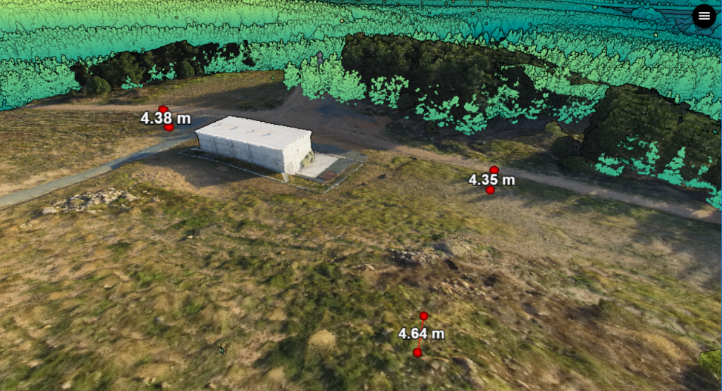
Using standard grid patterns (single or double), the point dataset showed less consistency across the area – which is a function of both ground control (none) and camera calibration (limited). The circular pattern offered incredibly good coincidence matching geometry for the entire dataset, making the life of photogrammetric reconstruction methods that much easier.
High oblique imagery
It would be remiss to not report on Anafi’s 180 gimbal capability – on one of my first few flights, I attempted to model a patio from above, around and under. Here’s a result:

…it isn’t the best outcome – ideally many more images would have contributed, but Anafi MK1 gave her gimbal for this flight partway through the planned image collection, and I’m not quite ready to try again. However, I’m quite happy with the potential – I can see under-eave (or other stucture) and internal space modelling in Anafi’s future, with a wiser pilot.
Anafilytics
We’ve collected some amazing pictures and pretty point clouds from a mini aircraft that is fun to fly. Now it’s time to do some observation/analysis with it.
Going back to our example of a small building survey, we have LiDAR from 2015 (interactive version here) and a half decent photogrammetric survey from 2018 (interactive version here) over the same patch of earth, with some significant change – we should be able to observe and measure what’s changed. Drawing on the data we’ve looked at above, we can see what the result might be:

…but because we care, we shall check somewhat more rigorously.
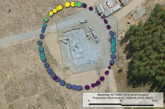
Using QGIS, define a region of interest to investigate based on the flight trajectory, which is extracted from the image EXIF tags:
exiftool -gpslatitude -gpslongitude -gpsaltitude -gpsxyaccuracy -gpszaccuracy mission4/images/*.JPG -c "%.8f" -n -csv > mission4geotags.csv…which gets us a neat .csv file we can import into QGIS (I’ve trimmed paths for clarity):
P0890592.JPG,-35.3139612858889,149.053296830028,618.7000122,0.503289192371533,0.779999971389771
P0890593.JPG,-35.3139533962778,149.053298682667,618.7000122,0.503289192371533,0.779999971389771
P0890594.JPG,-35.3139218073611,149.053308174139,618.7999878,0.495782228715942,0.779999971389771
P0890595.JPG,-35.3139004021667,149.053313825778,618.5999756,0.495782228715942,0.779999971389771
…and take a look. I’ve grabbed ACTMAPi’s 2018 aerial imagery as a base layer, and defined a polygon to investigate. We can see something is changing!
Next, use PDAL and entwine to define a process which lets us:
- clip out a matching chunk of data from the point cloud and the RPAS survey – which are both stored as cloud-based Entwine assets.
- align data, which are expressed with different heighting references
- create a ‘difference map’
The first step is to clip the point cloud parts we need, and determine a transformation matrix to align them. Remember – the two datasets are expressed in different vertical reference systems, one of which we need to more or less guess.
The 2015 data are height referenced to the Australian Height Datum (AHD); the 4.5-5m difference we see is a result of the RPAS survey being referenced to WGS84 + EGM96 heights (confirmed by Parrot).
We didn’t have that information at the time of processing – so a rigorous vertical datum transformation would have been a huge guess. Fortunately PDAL offers an iterative closest point (ICP) method to determine a rigid transformation between two point clouds – and may be a neat way of skipping over height datum transformation pain.
To avoid distractions, we limit the ICP filter to ground points – and stack our readers and filters into the PDAL pipeline below. Note how tags are used to hand different point views to stages:
{
"pipeline": [
    {
        "type": "readers.ept",
        "filename": "http://weston-mission4.s3.amazonaws.com/",
        "bounds": "([686672, 686725],[6090175, 6090232])",
        "tag": "rpas"
    },
    {
        "type": "readers.ept",
        "filename": "http://act-2015-rgb.s3.amazonaws.com/",
        "bounds": "([686672, 686725],[6090175, 6090232])",
        "tag": "lidar"
    },
    {
        "type": "filters.range",
        "inputs": "lidar",
        "limits": "Classification[2:2]",
        "tag": "lidargrnd"
    },
    {
        "type": "filters.smrf",
        "inputs": "rpas",
        "tag": "rpasclass"
    },
    {
        "type": "filters.range",
        "inputs": "rpasclass",
        "limits": "Classification[2:2]",
        "tag": "rpasgrnd"
    },
    {
        "type":"filters.icp",
        "inputs":[
                "lidargrnd",
                "rpasgrnd"
            ]
    }
]
}
…and our desired output is the transformation matrix produced by filters.icp, (note, no writers block is given) – so we invoke the pipeline as:
pdal pipeline clip-and-transform.json —metadata transform-result.json…which results in a lot more information that we really need. The part we want is a 16 element, space delimited array which represents a 4×4 transformation matrix flattened as row1->row2->row3->row4). This can be obtained by:
cat transform-result.json | jq .stages[].transformFrom here, every operation we do with the RPAS point dataset will have a transformation block applied. To clip our final comparison chunk from the RPAS dataset we use the pipeline:
{
"pipeline": [
    {
        "type": "readers.ept",
        "filename": "http://weston-mission4.s3.amazonaws.com/",
        "bounds": "([686672, 686725],[6090175, 6090232])"
    },
    {
        "type": "filters.smrf"
    },
    {
        "type": "filters.transformation",
        "matrix": "0.999989  2.18519e-06  -0.00511434     -2.89004-4.10424e-05     0.999974   -0.0074383      193.304  0.00511417   0.00743842     0.999961     -48817.9           0            0            0            1"
    },
    {
        "type": "filters.crop",
        "polygon": "POLYGON ((686691.444252 6090224.963413,686672.743588 6090217.629819,686678.060444 6090183.528609,686686.494076 6090176.011675,686721.511986 6090183.711949,686720.228607 6090219.096538,686706.111439 6090230.280268,686691.444252 6090224.963413))"
    },
    {
        "type": "writers.las",
        "filename": "rpas-transformed-subset.laz"
    }
]
}
…and from LIDAR – which is our reference point, and is already classified:
{
"pipeline": [
    {
        "type": "readers.ept",
        "filename": "http://act-2015-rgb.s3.amazonaws.com/",
        "bounds": "([686672, 686725],[6090175, 6090232])"
    },
    {
        "type": "filters.crop",
        "polygon": "POLYGON ((686691.444252 6090224.963413,686672.743588 6090217.629819,686678.060444 6090183.528609,686686.494076 6090176.011675,686721.511986 6090183.711949,686720.228607 6090219.096538,686706.111439 6090230.280268,686691.444252 6090224.963413))"
    },
    {
        "type": "writers.las",
        "filename": "lidar-clip.laz"
    }
]
}
Now that we have two point clouds we can check alignment/difference using CloudCompare. Here, I’ve offset the reference data by -20 m, and scaled the colours to show a range where most RPAS points sit – in the range -0.9 to +0.5 m in elevation from the reference dataset, after transformation. Given that the LiDAR uncertainty bounds are +-0.3m vertical against ground control, and the Anafi GPS accuracy was +-0.7m vertical, using the ICP approach to align data seems pretty good.

While this is a good check, it doesn’t yet help us achieve all our analytical objective. We can see that the Z offset is pretty constant across the RPAS dataset, which is a good sign – often uncontrolled RPAS models will have a slope/warp across the study region. We can see the obvious change – the building – and we can also see we’re pretty noise free. Which is nice.
We can see that the dirt road seen in both datasets slopes a touch more steeply in 2018, and that there is some change in ground level around the building. Referring back to our predictive sketch, we also want to know a bit more about the ground state change between 2015 and 2018. The building is a big distraction, so we’ll get rid of everything except ground and have a look.
Adding a filter block to our existing pipelines helps with this job:
{
    "type": "filters.range",
    "limits": "Classification[2:2]"
}
…and the results of a cloud to cloud difference in CloudCompare are given below:

…and we’re getting there! We can see that material has been removed (blue) near the building, and near the road – then added uphill of the building (orange/red). We also see some smaller change (subtraction of material) where the new roads are (dark green). For reference, here’s the 2018 state again, from the same perspective:

I was expecting to see greater material removal from the new road cut on the right – however, squinting and looking at the colour scale the magnitude of change is around 40cm, which rings true from walking around the site both pre-and post disturbance (local knowledge often helps!).
However, to be absolutely certain, we’d use rigorous ground control at collection time (Anafi is not RTK capable), and ensure a rigorous transformation to match vertical reference systems between the 2015 and 2018 surveys. We could also look at expressing both datasets on a common grid (rasterising) and creating a difference map to let us compute the volume of material shifted between the two surveys. A short post on that method may appear soon-ish (or as an update to this one).
Summary
The Anafi is a cute little machine, quiet, easy to fly, and suitable for actual geospatial work – given appropriate flight planning, position control and post-processing. I’ve shown here how six minutes in the air can turn into real geospatial insight – with appropriate care and data interpretation caveats.
As a first-time pilot, the Anafi has been pretty kind. It needs some caution around obstacles (best strategy – avoid). Parrot state that the lack of avoidance tech is to encourage people to fly within line of sight. My experience? Well, stay focussed while flying it. I think that’s an OK practice.
The aircraft is easy to fly, and so far behaves sanely if it gets confused mid-mission. I’ve flown in up to 25 km/h winds and it stays focussed/composed. And – it is quiet. In our age of excess noise, having an extra buzz overhead is never really welcome.
I’m looking forward to more data collection, testing, and operational deployment with Anafi, on the road toward larger aircraft, better cameras and airborne LiDAR.
…and we’ll get to the next parts of this series – terrestrial and mobile data, plus some basic mechanics – soon. Stay tuned!
The sales pitch
Spatialised is a fully independent, full time consulting business. The tutorials, use cases and write-ups here are free for you to use, without ads or tracking.
If you find the content here useful to your business or research, you can support production of more words and open source geo-recipes via Paypal or Patreon; or hire me to do stuff.