
Lidar datasets are big and sometimes hard to deal with. Its formats are daunting. There are a lot of ways to make it good, and also a lot to remember. This story is about some ways to help you when you get a pile of LAS files on your desk to deal with – or maybe just want to more about some data you have.
…without licenses or usage limitation issues.
Background: making sense of a lot of lidar
In 2017 I made an attempt at a web-based application named pointWPS for grabbing small chunks of just the data you need using open standards and data formats. It’s discussed here: The key issue wasn’t data size – we had a lot of space to put things – it was data and metadata quality.
All good data delivery systems begin with a catalogue, and catalogues are filled with metadata. Its crazy to store potentially trillions of things in a catalogue – put those things on a filesystem (which is already a catalogue – a really fast well optimised one), and put stuff about it into your searchable in-between layer.
For the pointWPS system this catalogue was a postGIS database. We extracted a bunch of metadata from thousands of lidar tiles we had on the filesystem and stuck it into the database – so we have enough data to find, and construct answers to spatial queries using postGIS. It turns out our metadata requirement was really close to STAC – although stuffed in a dynamic catalogue rather than a static metadata store.
This process found a lot of issues – missing coordinate systems, weird file namings, data that were not where they said they were. In turn, this sparked a lot of thinkering with PDAL and data/metadata querying for QA purposes. Without great metadata, we couldn’t add data to the catalogue; and in turn, we could not expose that data for analysis with pointWPS.
Since then, I’ve worked on other point cloud QA projects in the marine domain; and generally helped people fix things. This post is a cookbook of sorts resulting from that work. It focusses on ASPRS LAS format files, with a few examples for other data types to come later in the series.
What is PDAL?
PDAL is the Point Data Abstraction Library (https://pdal.io). It is designed to be a flexible tool for working with multiple point cloud formats, with a lot of add-ons and extensibility. It is single threaded, and not specifically designed to be the fastest point cloud processor. It does, however, offer you the ability to churn through points in many formats, and string together complex processing tasks easily.
You can install PDAL on Linux, MacOS and Windows, using the conda package manager or docker or native installation. Please note that each prepackaged distribution has slightly different sets of plugins included. If you head down the conda road be sure to use virtual environments – and try to use a single package source (conda-forge is great for PDAL things).
These examples are all made on a macOS laptop with PDAL installed via conda. I also have dockerised installations and a native installation in Ubuntu for various purposes.
If you’re not familiar at all with reading and writing data with PDAL, please go and read this tutorial first! The rest of this post covers very similar ground, with a skew toward providing pointers at processes which can be automated in Python
Tools for helping out
Because PDAL returns metadata as JSON, simple utilities can deliver results really efficiently. Python handles JSON output really easily, and in linux the very light jq utility helps sort out metadata returns. For ubuntu, grab it with:
#> sudo apt install jq…or using conda (in this case on MacOS X):
#> conda install -c conda-forge jqFor Pythonistas, the first code block I need to make the rest of this story happen looks like this:
import pdal
import json
import numpy as np
lasfile = “/path/to/inputfile.laz”

pipeline = [
        {
            "type": "readers.las",
            "filename": lasfile
        }
    ]

pipeline = pdal.Pipeline(json.dumps(pipeline))
pipeline.execute()
…which we assume exists for all following code snippets. The pipeline exists to read a las file and do nothing else, and we will assume it’s been run – so queries happen on the pipeline object.
Subject Data
This is the patch of points we’ll examine. It was collected in 2015 on behalf of the Australian Capital Territory Government. It has a contracted minimum point density of 8 points a square metre, and should be referenced to GDA94 / MGA zone 55 (EPSG:28355), with AHD heights (EPSG:5711). It has 2660756 points, is meant to be classified to ICSM level 3 (you’ll need to search this PDF to understand that) – and contains the wonderful National Museum of Australia – which you should visit if you get a chance. Click the image to explore the dataset it is clipped from:

Metadata examination
Because LAS files have comprehensive header structures, loads of QA questions can be answered without actually reading points.
pdal info is PDAL’s fundamental command line utility for asking questions about metadata and descriptive data statistics- it says ‘spew me all the LAS header plus some point statistics as JSON’. Give it a go, keep a note of all the fields it contains, then come back. This story is all about which parts of all that should we care about, and how do we get at them?
The pdal info application is documented here: https://pdal.io/apps/info.html – you’ll see we mainly use different option flags to get what we need in the command line – and similarly, use various filters to get just what we need in Python.
Let’s get started!
What is the data schema for my point cloud?
This tells us what data exists with each point (in PDAL, dimensions) in my point cloud. It’s a simple query to figure out if the things I thought I had are there…
#> pdal info inputfile.laz —schema# read the data schema from the pipeline object
pipeline.schemaBoth should return something like this – telling you all about what your LAS file contains and the data format each attribute (or dimension) has:
{
  "file_size": 21635653,
  "filename": "testclip2.laz",
  "now": "2020-05-02T15:19:49+1000",
  "pdal_version": "2.1.0 (git-version: Release)",
  "reader": "readers.las",
  "schema":
  {
    "dimensions":
    [
      {
        "name": "X",
        "size": 8,
        "type": "floating"
      },
      {
        "name": "Y",
        "size": 8,
        "type": "floating"
      },
      {
        "name": "Z",
        "size": 8,
        "type": "floating"
      },
      {
        "name": "Intensity",
        "size": 2,
        "type": "unsigned"
      },
      {
        "name": "ReturnNumber",
        "size": 1,
        "type": "unsigned"
      },
      {
        "name": "NumberOfReturns",
        "size": 1,
        "type": "unsigned"
      },
      {
        "name": "ScanDirectionFlag",
        "size": 1,
        "type": "unsigned"
      },
      {
        "name": "EdgeOfFlightLine",
        "size": 1,
        "type": "unsigned"
      },
      {
        "name": "Classification",
        "size": 1,
        "type": "unsigned"
      },
      {
        "name": "ScanAngleRank",
        "size": 4,
        "type": "floating"
      },
      {
        "name": "UserData",
        "size": 1,
        "type": "unsigned"
      },
      {
        "name": "PointSourceId",
        "size": 2,
        "type": "unsigned"
      },
      {
        "name": "GpsTime",
        "size": 8,
        "type": "floating"
      },
      {
        "name": "ScanChannel",
        "size": 1,
        "type": "unsigned"
      },
      {
        "name": "ClassFlags",
        "size": 1,
        "type": "unsigned"
      },
      {
        "name": "Red",
        "size": 2,
        "type": "unsigned"
      },
      {
        "name": "Green",
        "size": 2,
        "type": "unsigned"
      },
      {
        "name": "Blue",
        "size": 2,
        "type": "unsigned"
      },
      {
        "name": "OriginId",
        "size": 4,
        "type": "unsigned"
      }
    ]
  }
}
What LAS format am I looking at?
Related to the data schema, it is useful to know about a LAS file’s version and data format. Those can be found using:
#> pdal info —metadata | jq .metadata.minor_version
#> pdal info —metadata | jq .metadata.pointformat_id
In Python, we use the JSON library to extract the same data.
# query JSON metadata from the pipeline object for LAS minor version
json.loads(pipeline.metadata)["metadata"]["readers.las"]["minor_version”]

# query JSON metadata from the pipeline object for LAS data format
json.loads(pipeline.metadata)["metadata"]["readers.las"]["dataformat_id"]
These queries will return numbers. Our minor_version is 4 and dataformat_id is 6.
Your data schema (the first query) should match the ASPRS specifications for your combination of LAS minor version and dataformat ID. If you are doing QA programatically, you could assemble a dictionary of dimensions you’d expect for a given format. LAS 1.4 is trickier, since things get flexible and we have user defined dimensions allowed. There, just make sure you know what to expect!
Examining the metadata element of pdal info —metadata returns gives you a number of other quick checks – extents in three dimensions, scales and offsets, and a point count. As well as georeferencing information.
These are all accessible using the same strategy. Using point count (does my LAS file even have points?) as an example, we’d do:
#> pdal info inputfile.laz —metadata | jq .metadata.count# query JSON metadata from the pipeline object for point count
json.loads(pipeline.metadata)["metadata"]["readers.las"]["count"]…again these queries will return a number – in this case 2660756. If they return 0, you probably have problems…
Note – PDAL’s metadata querying doesn’t offer up a density estimate . It’s really inaccurate to infer density based on point count and min/max bounding boxes. We will get to density – with better methods.
Where on earth are my points?
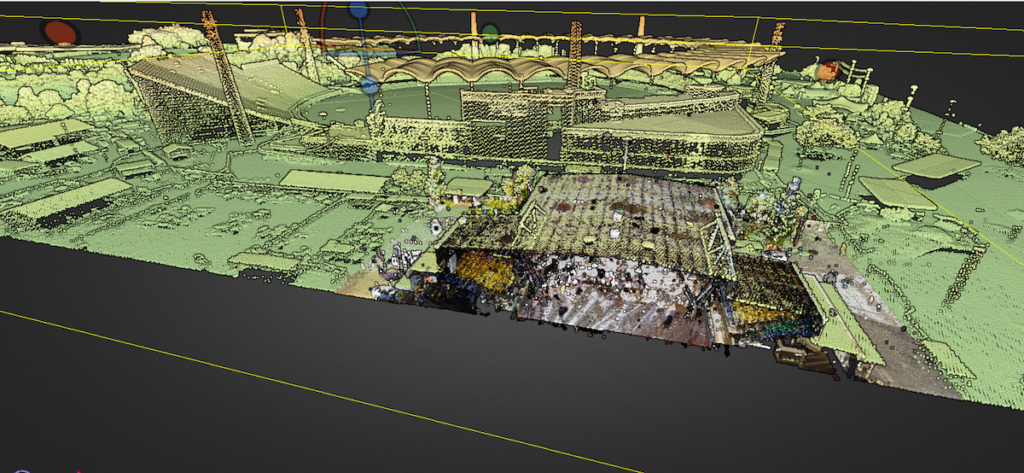
Having reference frame data is essential, even for TLS collections – it’s imperative to know where the data are in the world, because you might want to combine it with something else later. In the image here, a huge TLS scan of a stadium is registered with an airborne survey – which was very difficult because the TLS scanner did not collect georeferencing data up front.In short, georeference your data!
Accessing SRS data happens via the —metadata flag on pdal info at the command line:
#> pdal info inputfile.laz —metadata This spews a lot of information out about all kinds of things. We can filter things to ‘do I have a CRS’ using jq or Python:
#> pdal info inputfile.laz —metadata | jq .metadata.srs.horizontal…which gives us a bunch of WKT, rather than a neat EPSG code – but at least you can see there’s a crs! Looking for a vertical CRS, use:
#> pdal info inputfile.laz —metadata | jq .metadata.srs.verticalThese both return OGC WKT describing EPSG:28355 and EPSG:5711. I tried piping results to gdalsrsinfo and ogr2ogr, but haven’t found the magical combination yet to extract just EPSG codes on the command line.
In python using a helper application osr makes life simpler – we can get EPSG codes (if we have PDAL python, we already have osr because it is a PDAL dependency). Here, we pass WKT straight to osr and get back an EPSG number:
import osr

horz_srs = osr.SpatialReference(metadata["metadata"]["readers.las"]["srs"]["horizontal”])
horz_epsg = horz_srs.GetAttrValue("AUTHORITY", 1)

vert_srs = osr.SpatialReference(metadata["metadata"]["readers.las"]["srs”]["vertical”])
vert_epsg = vert_srs.GetAttrValue("AUTHORITY", 1)
In this verstion, we get back two numbers: 28355 and 5711. If you’re after proj strings or something else, dig into osr and its coordinate system manipulation tooling.
In a QA sense, it should be a hard ‘return to vendor’ if, at a minimum, horizontal CRS data are missing or incorrect for any laser scanning data. Requiring a vertical CRS will also help you a lot in future, when we all shift to dynamic datums and you’re trying to sort out weird misalignments…
Once we’ve exhausted header data for information, we need to start reading points from our LAS files…
Querying points to discover things
These processes take longer, since we are querying some or all of the points. Most of the time input LAS files (and some other data types) have internal organisation by time, or some other attribute rather than spatial coherence. If you’ve got time, sometimes running pdal sort (or using filters.mortonorder ) to preprocess data can really help downstream, although its pretty time consuming up front.
Statistics on dimensions
pdal info gives us a huge spew of information on each dimension with descriptive statistics. You can narrow those down using the —dimensions flag in a shell script:
#> pdal info inputfile.laz --dimensions X,Y,Z…will net you JSON output giving summary statistics for the listed values, in this case X, Y and Z (see your schema dump for hints about what you can find in there).
This is sort of useful to see what’s there – however, you may want to get finer detail. A couple of common questions might be ‘what classification labels exist?’; or ‘how many returns / return numbers do we have?’.
We can use filters.stats to help here:
#> pdal info inputfile.laz --dimensions Classification --filters.stats.count=Classification

#> pdal info inputfile.laz --dimensions ReturnNumber --filters.stats.count=ReturnNumber
In Python we need to extend the pipeline a little, adding a filters.stats block:
pipeline = [
        {
            "type": "readers.las",
            "filename": lasfile
        },
        {   "type": "filters.stats",
            "dimensions": "Classification,ReturnNumber,NumberOfReturns",
            "count": "Classification,ReturnNumber,NumberOfReturns"}
    ]

pipeline = pdal.Pipeline(json.dumps(pipeline))
pipeline.execute()
When we get our blob of JSON back we’ll have an extra filters.stats element which we interrogate like this:
#load the metadata string into a dictionary and query it...
json.loads(infopipeline.metadata)["metadata"]["filters.stats”]["statistic"]
You’ll see that this returns an array! Our pipeline could have collected counts of every dimension, but then you need to dig into a list to find it – so limiting output makes sense for humans. For machines, something like this could work:
#load up a list with statistics on dimensions
stats = json.loads(infopipeline.metadata)["metadata"]["filters.stats"]["statistic”]

#name our statistic of interest
stat_of_interest = “Classification"

#…and a short list comprehension nets a result!
[s for s in stats if s["name"]==stat_of_interest]
…which will return something like this, depending on your input data:
[{'average': 3.956180123,
  'count': 2660756,
  'counts': ['1.000000/1595',
   '2.000000/649495',
   '3.000000/773555',
   '4.000000/57141',
   '5.000000/825982',
   '6.000000/210419',
   '7.000000/625',
   '9.000000/141660',
   '17.000000/235',
   '18.000000/49'],
  'maximum': 18,
  'minimum': 1,
  'name': 'Classification',
  'position': 2,
  'stddev': 1.802507636,
  'variance': 3.249033776}]
Using the counts element, you have a neat histogram of how many points you have in each Classification. And we can see more or less what we’d expect here. Looking at ReturnNumber is also informative:
[{'average': 1.336544952,
  'count': 2660756,
  'counts': ['1.000000/2021797',
   '2.000000/428946',
   '3.000000/168572',
   '4.000000/36744',
   '5.000000/4356',
   '6.000000/328',
   '7.000000/13'],
  'maximum': 7,
  'minimum': 1,
  'name': 'ReturnNumber',
  'position': 0,
  'stddev': 0.6746167124,
  'variance': 0.4551077086}]
For these we’re not really super keen on descriptive statistics, we want the counts! For other dimensions, you might want something different.
These fairly straightforward statistical queries provide another pass/fail point for QA – its simple to asses whether classes exist in the data. It doesn’t validate classification labelling – just lets you know that you have classifications if you paid for them!
Point density
Point density always varies across a lidar collection – and is usually a key deliverable (eg N points per square unit). Measuring density using bounding boxes is fraught – since we don’t always have full coverage across a box. We can overcome this using PDAL’s filters.hexbin – which uses a hexagonal binning strategy to estimate point coverage and density. This way, we get a more realistic answer to ‘in the lidar coverage, what is the average point density?‘
pdal info has a --boundary flag to drive filters.hexbin as a bash one-liner. Before we start! Because filters.hexbin tries to guess what want, we should help it out with some idea of how close we want our density estimate to be. For this query it’s a pretty small area so we will make smallish hexagons, using an edge length of 10 units (metres).
#> pdal info inputfile.laz —boundary —filters.hexbin.edge_length=10 | jq .boundary.densityIn Python we need to add filters.hexbin to our pipeline to get a density estimate:
pipeline = [
{
"type": “readers.las",
"filename": lasfile
},
{
"type": “filters.hexbin”,
"edge_length”: 10
}
]

pipeline = pdal.Pipeline(json.dumps(pipeline))
pipeline.execute()
json.loads(infopipeline.metadata)["metadata"]["filters.hexbin"]["density”]
Both the command line and python versions here report back a single number – mean point density as `(number of points inside the hexbin boundary)/(area of hexbin boundary)`, which for the test data at the hexbin resolution used is 10.27ish. So – great! The vendor has definitely met the 8ppm mark.
Ideally, to avoid vendor frustration, we should QA this metric with a boundary as close to the desired coverage as possible. I purposefully picked a test dataset with water (returns we don’t really use or want), just to make life a little more interesting.
As a note – we could have done all the other QA tasks above with filters.hexbin in place. Now you know about it, you can build it into your own metadata pipelines from the start!
From a QA point of view this is a starting point. filters.hexbin uses a sample of points to decide the boundary ‘resolution’, which may need tweaking. Further, average density over some survey area can be highly skewed! So you have a pile of decisions ahead about what you need to do to apply these tools.
In part two of this series, we’ll look at finding and reporting on where surveys are more or less dense – and using the boundaries created to do some other QA tasks (like coverage testing)
What about 3D density?
…these are so far oriented at a two dimensional construct of ‘coverage’. What about the 3rd dimension? What is the 3D density of our point cloud? We can use filters.radialdensity to discover that – combined with filters.voxelgrid to trim down the number of points we have to deal with at the end – and obtain an indication of how many points per cubic metre exist. filters.radialdensity adds a new dimension to the point cloud being examined. The process in bash is a little convoluted – you need to write out a new file in a format which could handle an extraradialdensity dimension (eg a LAS 1.4 extra dimension), and then examine it with pdal info. Here, I want an approximation of points per cubic metre, so my radius is set to 0.6204m. This took 39 seconds to process 2.6 million points – it’s a bit slower than metadata reading or hex binning!
#> pdal translate inputfile.laz radialdensityfile.laz radialdensity --filters.radialdensity.radius=0.6204 --writers.las.minor_version=4 --writers.las.extra_dims=all

#> pdal info --dimensions RadialDensity radialdensityfile.laz
This returns:
{
  "file_size": 29035048,
  "filename": "radialdensityfile.laz",
  "now": "2020-05-02T15:01:45+1000",
  "pdal_version": "2.1.0 (git-version: Release)",
  "reader": "readers.las",
  "stats":
  {
    "statistic":
    [
      {
        "average": 10.30846558,
        "count": 2660756,
        "maximum": 32.99212811,
        "minimum": 0.9997614579,
        "name": "RadialDensity",
        "position": 0,
        "stddev": 5.30121048,
        "variance": 28.10283255
      }
    ]
  }
}
…giving an average 3D density of 10.3ish points per cubic-metre-surrounding-each-point. Importantly this is not a count of points per ‘cubic metre voxel’, it’s a normalised count of points (count / volume) in a sphere around every point in the LAS file.
In python, we do this like:
densitypipeline = [
        {
            "type": "readers.las",
            "filename": lasfile
        },
        {
            "type": "filters.radialdensity",
            "radius": 0.6204
        }

    ]

densitypipeline = pdal.Pipeline(json.dumps(densitypipeline))
densitypipeline.execute()

#we haven’t used numpy yet, here it is…
# this also shows accessing a PDAL dimension from structured arrays
# which are generated to hold data!
np.mean(densitypipeline.arrays[0]['RadialDensity'])
Again this gives us the mean 3D density using a sphere of one cubic metre around each point.
PDAL has some voxel manipulation tools for filtering, if voxels are your thing – but they (as yet) don’t keep per-voxel point statistics (please talk to Hobu Inc about applying cash to that capability if it sounds useful!
Wrapping up
In this wander through some functional QA tasks with PDAL we’ve covered a lot of metadata inspection and some data introspection using both Python and a command line interface, with some neat tooling for inspecting results.
This has provided the bones for mostly-automated lidar QA using open tools – not to mention helping with any manual inspection you need to do. I’ll update this post soon with an interactive notebook stepping through all of the QA tasks given here. Heading into some automation, because all the software is openly licensed your only limitation is your ability to consume (and pay for) CPUS and RAM. If you have 1000 las tiles, you could run QA tasks on them all in one hit given 1000 small computers and some glue to drive them.
We are not done yet though! Part of data QA involves using other datasets to help examine where our data sit in the world and how well they sit there. Part two will look at testing coverages, and comparison against reference targets. And perhaps a few more things.
Of course, while I’ve tested and retested whats here there are probably at least a few bugs in there. Please reach out if you find any!
Credits
All of this is made possible by the open source geospatial community and in particular Hobu Inc, the primary maintainers of PDAL and associated tooling. The ACT Government released its 2015 lidar+imagery survey as completely open data, which means Spatialised got to colourise all the points and build an awesome open data source with it.
Thanks everyone!
The sales pitch
Spatialised is a fully independent consulting business. Everything you see here is open for you to use and reuse, without ads. WordPress sets a few cookies for statistics aggregation, we use those to see how many visitors we got and how popular things are.
If you find the content here useful to your business or research or billion dollar startup idea, you can support production of ideas and open source geo-recipes via Paypal, hire me to do stuff; or hire me to talk about stuff.