
This is part 1 of 3, explaining how uncertainties in lidar point geolocation can be estimated for one type of scanning system. We know lidar observations of elevation/range are not exact (see this post), but a critical question of much interest to LiDAR users is ‘how exact are the measurements I have’?
As an end-used of lidar data I get a bunch of metadata that is provided by surveyors. One of the key things I look for are the accuracy estimates. Usually these come as some uncertainty in East, North and Up measurements, in metres, relative to the spatial reference system the point measurements are expressed in. What I don’t get is any information about how these figures are arrived at, or if they apply equally to every point. It’s a pretty crude measure.
As a lidar maker, I was concerned with the uncertainty of each single point – particularly height – because I use these data to feed a model for estimating sea ice thickness. I also need to feed in an uncertainty – so that I can put some boundaries around how good my sea ice thickness estimate is. However, there was no way of doing so in an off the shelf software package – so I implemented the lidar geoferencing equations and a variance-covariance propagation method for them in MATLAB and used these. This was a choice of convenience at the time, and I’m now (very) slowly porting my code to Python, so that you don’t need a license to make lidar points and figure out their geolocation uncertainties.
My work was based on two pieces of fundamental research: Craig Glennie’s work on rigorous propagation of uncertainties in 3D [1], and Phillip Schaer’s implementation of the same equations [2]. Assuming that we have a 2D scanner, the lidar georeferencing equation is:
![\begin{bmatrix} x \\ y \\ z \\ \end{bmatrix}^m= \begin{bmatrix} X\\ Y\\ Z\\ \end{bmatrix} + R^b_m \left[ R^b_s \rho \left( \begin{gathered} sin\Theta\\ 0\\ cos\Theta \end{gathered} \right) + \begin{bmatrix} a_x\\ a_y\\ a_z\\ \end{bmatrix}^b \right]](https://s0.wp.com/latex.php?latex=%5Cbegin%7Bbmatrix%7D+x+%5C%5C+y+%5C%5C+z+%5C%5C+%5Cend%7Bbmatrix%7D%5Em%3D+%5Cbegin%7Bbmatrix%7D+X%5C%5C+Y%5C%5C+Z%5C%5C+%5Cend%7Bbmatrix%7D+%2B+R%5Eb_m+%5Cleft%5B+R%5Eb_s+%5Crho+%5Cleft%28+%5Cbegin%7Bgathered%7D+sin%5CTheta%5C%5C+0%5C%5C+cos%5CTheta+%5Cend%7Bgathered%7D+%5Cright%29+%2B+%5Cbegin%7Bbmatrix%7D+a_x%5C%5C+a_y%5C%5C+a_z%5C%5C+%5Cend%7Bbmatrix%7D%5Eb+%5Cright%5D&bg=ffffff&fg=000&s=0&c=20201002)
The first term on the right is the GPS position of the vehicle carrying the lidar:

The next term is made up of a few things. Here we have points in lidar scanner coordinates (relative to instrument axes):

…which means ‘range from scanner to target’ (


Note that there is no Y coordinate! This is a 2D scanner, observing an X axis (across track) and a Z axis (from ground to scanner). The Y coordinate is provided by the forward motion of a vehicle, in this case a helicopter.
For a 3D scanner, or a scanner with an elliptical scan pattern, there will be additional terms describing where a point lies in the instrument reference frame. Whatever term is used at this point, the product is the position of a reflection-causing object in the instrument coordinate system which is rotated to the coordinate system of the vehicle’s navigation device using the matrix:

The point observed also has a lever arm offset added (the distance in 3 axes between the navigation device’s reference point and the laser scanner’s reference point), so we pretend we’re putting our navigation device exactly on the instrument reference point:

This mess of terms is finally rotated to a mapping frame using euler angles in three axes (essentially heading, pitch, roll) recorded by the navigation device:

…and added to the GPS coordinates of the vehicle (which are really the GPS coordinates of the navigation system’s reference point).
There are bunch of terms there – 14 separate parameters which go into producing a point, and that’s neglecting beam divergence plus only showing single returns. Sounds crazy – but the computation is actually pretty efficient.
Here’s a diagram of the scanner system I was using – made from a 3D laser scan and some engineering drawings. How’s that? Using a 3D scanner to measure a 2D scanner. Even better, the scan was done on the helipad of a ship in the East Antarctic pack ice zone!
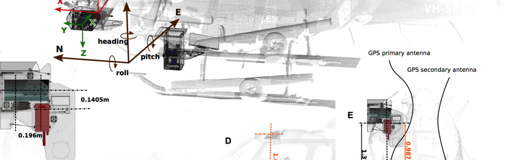
You can see there the relationships I’ve described above. The red box is our navigation device – a dual-GPS, three-axis-IMU strapdown navigator, which provides us with the relationship between the aircraft body and the world. The green cylinder is the laser scanner, which provides us ranges and angles in its own coordinate system. The offset between them is the lever arm, and the orientation difference between the axes of the two instruments is the boresight matrix.
Now consider that each of those parameters from each of those instruments and the relationships between them have some uncertainty associated with them, which contributes to the overall uncertainty about the geolocation of a given lidar point.
Mind warped yet? Mine too. We’re all exhausted from numbers now, so part 2 examines how we take all of that stuff and determine, for every point, a geolocation uncertainty.
Feel free to ask questions, suggest corrections, or suggest better ways to clarify some of the points here.
There’s some code implementing this equation here: https://github.com/adamsteer/LiDAR-georeference – it’s Apache 2.0 licensed and matlab, and in some years now I haven’t really touched it. Feel free to fork the code and make pull requests to get it all working, robust and community-driven!
Meanwhile, read these excellent resources:
[1] Glennie, C. (2007). Rigorous 3D error analysis of kinematic scanning LIDAR systems. Journal of Applied Geodesy, 1, 147–157. http://doi.org/10.1515/JAG.2007. (accessed 19 January 2017)
[2] Schaer, P., Skaloud, J., Landtwing, S., & Legat, K. (2007). Accuracy estimation for laser point cloud including scanning geometry. In Mobile Mapping Symposium 2007, Padova. (accessed 19 January 2017)
The sales pitch
Spatialised is a fully independent consulting business. Everything you see here is open for you to use and reuse, without ads. WordPress sets a few cookies for statistics aggregation, we use those to see how many visitors we got and how popular things are.
If you find the content here useful to your business or research or billion dollar startup idea, you can support production of ideas and open source geo-recipes via Paypal, hire me to do stuff; or hire me to talk about stuff.