
Lidar is a pretty common tool for geospatial stuff. It means ‘Light Detection and Ranging’. For the most part involved shining a laser beam at something then measuring how long a reflection takes to come back. Since we approximate the speed of light, we can use the round trip time to estimate the distance between the light source and ‘something’ with a great degree of accuracy. Modern instruments perform many other types of magic – building histograms of individual photons returned, comparing emitted and returned wave pulses, and even doing this with many different parts of the EM spectrum.
Take a google around about lidar basics – there are many resources which already exist to explain all this, for example https://coast.noaa.gov/digitalcoast/training/intro-lidar.html.
What I want to write about here is a characteristic of the returned point data. A decision that needs to be made using lidar is:
Where should I measure a surface?
…but what – wait? Why is this even a question? Isn’t lidar just accurate to some figure?
Sort of. A few years ago I faced a big question after finding that the lidar I was working on was pretty noisy. I made a model to show how noisy the data should be, and needed some data to verify the model. So we hung the instrument in a lab and measured a concrete floor for a few hours.
Here’s a pretty old plot of what we saw:
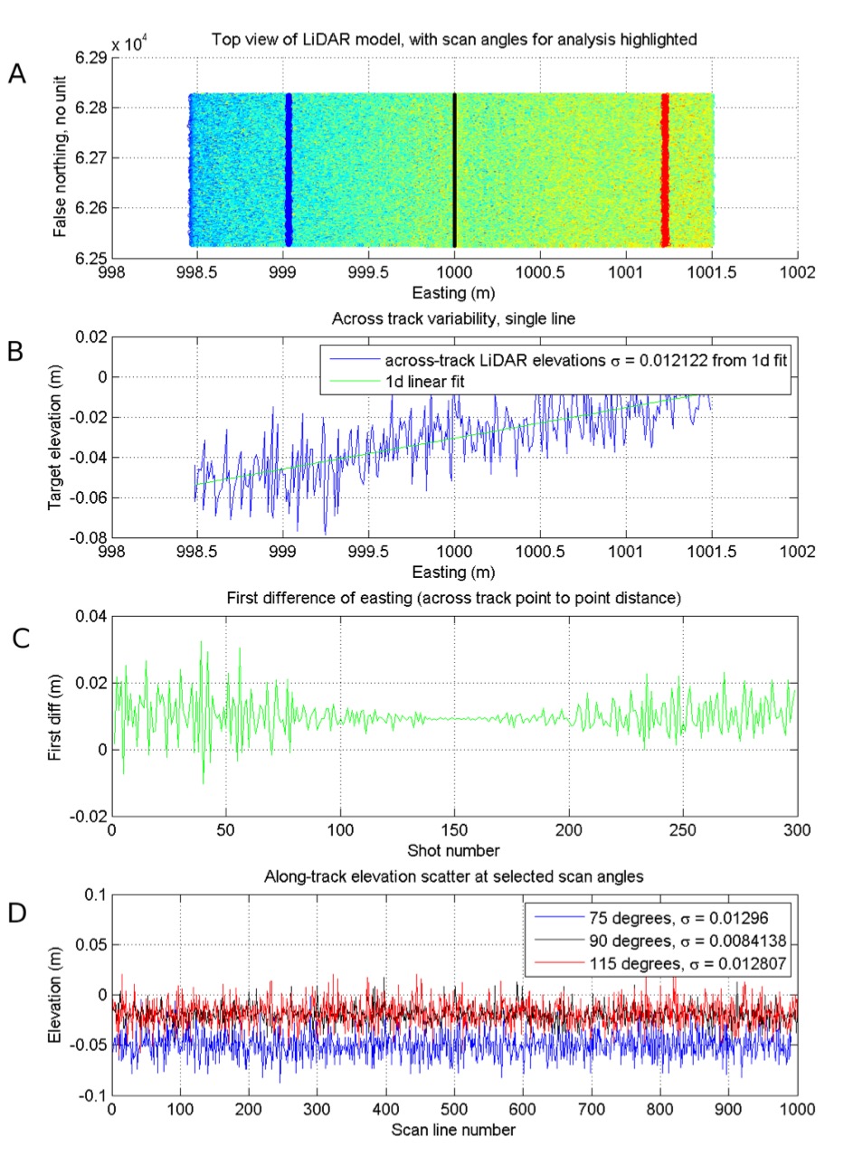
What’s going on here? In the top panel, I’ve spread our scan lines along an artificial trajectory heading due north (something like N = np.arange(0,10,0.01)), with the Easting a vector of zeroes and height a vector of 3’s – and then made a swath map. I drew in lines showing where scan angle == 75, 90, and 115 are.
In the second panel (B), there’s a single scanline show across-track. This was kind of a surprise – although we should have expected it. What we see is that the range observation from the lidar is behaving as specified – accurate to about 0.02 m (from the instrument specifications). What we didn’t realise was that accuracy is angle-dependent, since moving away from instrument nadir the impact of angular measurement uncertainties becomes greater than the ranging uncertainty of the instrument.
Panels C and D show this clearly – near instrument nadir, ranging is very good! Near swath edges we approach the published instrument specification.
This left us with the question asked earlier:
When we want to figure out a height reference from this instrument, where do we look?
If we use the lowest points, we measure too low. Using the highest points, we measure too high. In the end I fitted a surface to the points I wanted to use for a height reference – like the fit line in panel B – and used that. Here is panel B again, with some annotations to help it make sense.

You can see straight away there are bears in these woods – what do we do with points which fall below this plane? Throw them away? Figure out some cunning way to use them?
In my case, for a number of reasons, I had to throw them away, since I levelled all my points using a fitted surface, and ended up with negative elevations in my dataset. Since I was driving an empirical model based on these points, negative input values are pretty much useless. This is pretty crude. A cleverer, more data-preserving method will hopefully reveal itself sometime!
I haven’t used many commercial lidar products, but one I did use a reasonable amount was TerraSolid. It worked on similar principles, using aggregates of points and fitted lines/planes to do things which required good accuracy – like boresight misalignment correction.
No doubt instruments have improved since the one I worked with. However, it’s still important to know that a published accuracy for a lidar survey is kind of a mean (like point density) – some points will have a greater chance of measuring something close to where it really is than others. And that points near instrument nadir are more likely to be less noisy and more accurate.
That’s it for now – another post on estimating accuracy for every single lidar point in a survey will come soon(ish).
To finish with, Martin Isenburg has an excellent related post on ‘fluffy lidar’ here: https://rapidlasso.com/2017/10/29/processing-drone-lidar-from-yellowscans-surveyor-a-velodyne-puck-based-system/
Enjoy – and I hope this helps!
The figure shown here comes from an internal technical report I wrote in 2012. Data collection was undertaken with the assistance of Dr Jan L. Lieser and Kym Newbery, at the Australian Antarctic Division. Please contact me if you would like to obtain a copy of the report – which pretty much explains this plot and a simulation I did to try and replicate/explain the lidar measurement noise.
The sales pitch
Spatialised is a fully independent consulting business. Everything you see here is open for you to use and reuse, without ads. WordPress sets a few cookies for statistics aggregation, we use those to see how many visitors we got and how popular things are.
If you find the content here useful to your business or research or billion dollar startup idea, you can support production of ideas and open source geo-recipes via Paypal, hire me to do stuff; or hire me to talk about stuff.