In part 1, we looked at one way that a lidar point is created. Just to recap, we have 14 parameters (for the 2D scanner used in this example) each with their own uncertainty. Now, we work out how to determine the geolocation uncertainty of our points.
First, let’s talk about what those uncertainties are. An obvious target is GPS positioning uncertainty, and this is the source that comes to mind first. Using a dual-frequency GPS gives the advantage of sub-decimetre positioning, after some post-processing is done. Merging those positions with observations from the IMU constrains those positions even further.
For a quick mental picture of how this works, consider that the navigation unit is collecting a GPS fix every half a second. The accelerometers which measure pitch, roll and heading take a sample every 1/250th of a second. They also keep track of how far they think they’ve moved since the last GPS fix – plus the rate of motion is tracked, putting a limit on how far it is possible to move between each GPS fix. The navigation unit compares the two data sources. If the GPS fix is wildly unexpected, a correction is added to GPS positions and we carry on.
So we get pretty accurate positions (~5cm).
But is that the uncertainty of our point positions? Nope. There’s more. The laser instrument comes with specifications about how accurate laser ranging is, and how accurate it’s angular encoder is.
Even more, the navigation device has specifications about how accurate it’s accelerometers are, and all of these uncertainties contribute! How?
Variance-covariance propagation to the rescue
Glennie [1] and Schaer [2] used Variance-covariance propagation to estimate the uncertainty in geolocation of LiDAR points. This sounds wildly complex, but at it’s root is a simple idea:
See that? we figured out the uncertainty of a thing made from adding thing1 and thing2, by knowing what the uncertainties of things1 and thing2 are.
Going from simple addition to a few matrix multiplications was a quantum leap, handled neatly by symbolic math toolboxes – but only after I nearly quit my PhD trying to write out the uncertainty equation by hand.
Here is the uncertainty equation for lidar points, whereis the uncertainty:
What!! Is that all? I’m joking, right?
Nearly. is a 14-element vector containing partial derivatives of each the parameters that go into the lidar georeferencing equation (the so-called Jacobians).
is a 14 x 14 matrix on which the uncertainties associated with each element occupy the diagonal.
Writing this set of equations out by hand was understandably a nightmare, but more clever folks than myself have achieved it – and while I certainly learned a lot about linear algebra in this process, I took advice from an old astronomer and used a symbolic maths toolbox to derive the Jacobians.
…which meant that the work actually got done, and I could move on with research!
Now my brain is fully exploded – what do uncertainties look like?
Glennie [1] and Schaer [2] both report that at some point, angular motion uncertainty overtakes GPS position uncertainty as the primary source of doubt about where a point is. Fortunately I found the same thing. Given the inherent noise of the system I was using, this occurred pretty quickly. In the Kalman filter which integrates GPS and IMU observations, a jittery IMU is assigned a higher uncertainty at each epoch. This makes sense, but also means that angular uncertainties need to be minimised (for example, by flying instruments in a very quiet aircraft or an electric-powered UAS)
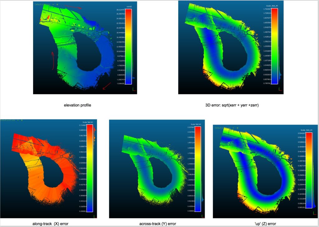
I made the following map to check that I was getting georeferencing right, and also getting uncertainty estimates working properly.
It could be prettier, but you see how the components all behave – across-track and ‘up’ uncertainties are dominated by the angular component not far off nadir. Along-track uncertainties are more consistent across-track, because the angular measurement components (aircraft pitch and a bit of yaw) are less variable.
The sample in the next section shows point elevation uncertainties (relative to an ITRF08 ellipsoid) during level flight over sea ice. At instrument nadir, height uncertainty is more or less equivalent to instrument positioning uncertainty. Increasing uncertainties toward swath edges are a function of angular measurement uncertainty.
But normally LiDAR surveys come with an averaged accuracy level. Why bother?
i. why I bothered:
In a commercial survey the accuracy figure is determined mostly by comparing lidar points with ground control data – and the more ground control there is, the better (you have more comparison points and can make a stronger estimate of the survey accuracy).
Over sea ice this is impossible. I was also using these points as input for an empirical model which attempts to estimate sea-ice thickness. As such, I needed to also propagate uncertainties from my lidar points through the model to sea-ice thickness estimates.
In other words, I didn’t want to guess what the uncertainties in my thickness estimates were. As far as plausible, I need to know what the input uncertainty is for each thickness estimate is – so every single point. It’s nonsensical to suggest that every observation and therefore every thickness estimate comes with the same level of uncertainty.
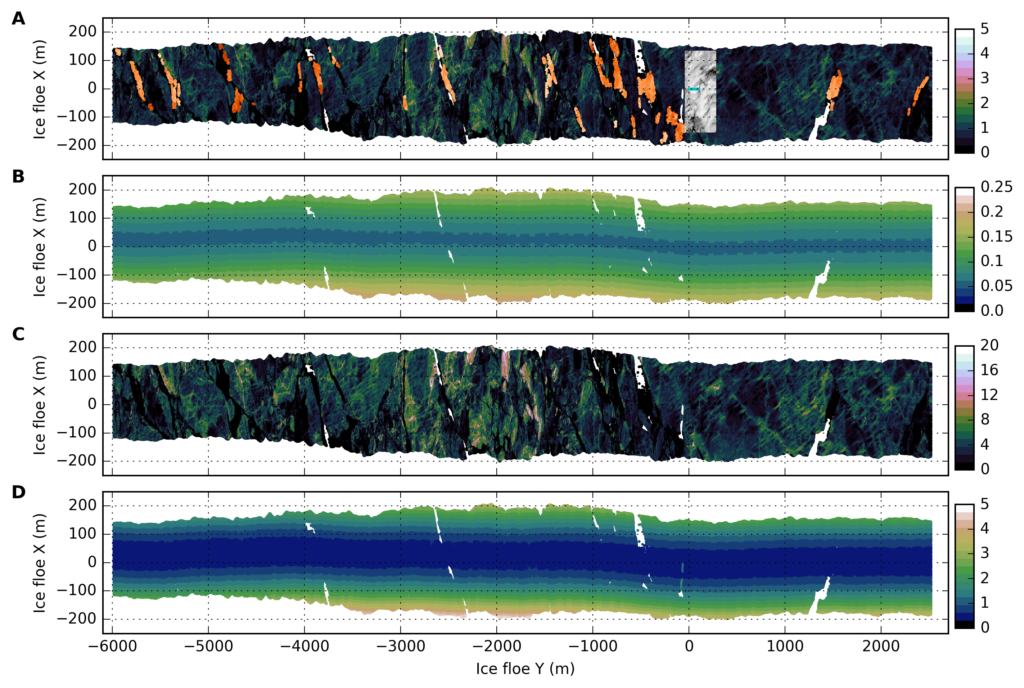
Here is another map from my thesis. It’s pretty dense, but shows the process in action:
The top panel is ‘height above sea level’ for sea ice. Orange points are ‘sea level reference’ markers, and the grey patch highlights an intensive survey plot. The second panel is uncertainty associated with each height measurment. In panel three we see modelled sea ice thickness (I’ll write another post about that later), and the final panel shows the uncertainty associated with each thickness estimate. Thickness uncertainties are greater than height uncertainties because we’re also accounting for uncertainties in each of the other model parameters (lidar elevations are just one). So, when I get to publishing sea-ice thickness estimates, I can put really well made error bars around them!
ii. why you, as a commercial surveyor or an agency contracting a LiDAR survey or a LIDAR end user should bother:
The computation of uncertainties is straightforward and quick once the initial figuring of the Jacobians is done – and these only need to be recomputed when you change your instrument configuration. HeliMap (Switzerland) do it on-the-fly and compute a survey quality metric (see Schaer et al, 2007 [2]) which allows them to repeat any ‘out of tolerance’ areas before they land. Getting an aircraft in the air is hard, and keeping it there for an extra half an hour is easy – so this capability is really useful in terms of minimising costs to both contracting agencies and surveyors. This analysis in conjunction with my earlier post on ‘where exactly to measure in lidar heights‘ shows you where you can assign greater confidence to a set of lidar points.
It’s also a great way to answer some questions – for example are surveyors flying over GCP’s at nadir, and therefore failing to meet accuracy requirements off-nadir? Are critical parts of a survey being captured off-nadir, when it would be really useful to get the best possible data over them? (this has implications for flight planning). As a surveyor, this type of thinking will give you fewer ‘go back and repeat’ jobs – and as a contracting agency, you might spend a bit more on modified flight plans, but not a lot more to get actually really great data instead of signing off and then getting grief from end users.
As an end user of lidar products, If you’re looking for data quality thresholds – for example ‘points with noise < m over a flat surface’, this type of analysis will help you out. I’ve also talked to a number of end users who wonder about noisy flight overlaps, and why some data don’t appear to be well-behaved. Again, having some quality metric around each point will help an end-user determine which data are useful, and which should be left alone.
Summarising
I certainly stand on the shoulders of giants here, and still incur brain-melting when I try to come at these concepts from first-principles (linear algebra is still hard for me!). However, the idea of being able to estimate in an a-priori quality metric is, in my mind, really useful.
I don’t have much contact with commercial vendors, so I can only say ‘this is a really great idea, do some maths and make your lidar life easer!’.
I implemented this work in MATLAB, and you can find it here:
https://github.com/adamsteer/LiDAR-georeference
With some good fortune it will be fully re-implemented in Python sometime. Feel free to clone the repository and go for it. Community efforts rock!
And again, refer to these works:
[1] Glennie, C. (2007). Rigorous 3D error analysis of kinematic scanning LIDAR systems. Journal of Applied Geodesy, 1, 147–157. http://doi.org/10.1515/JAG.2007. (accessed 19 January 2017)
[2] Schaer, P., Skaloud, J., Landtwing, S., & Legat, K. (2007). Accuracy estimation for laser point cloud including scanning geometry. In Mobile Mapping Symposium 2007, Padova. (accessed 19 January 2017)
The sales pitch
Spatialised is a fully independent consulting business. Everything you see here is open for you to use and reuse, without ads. WordPress sets a few cookies for statistics aggregation, we use those to see how many visitors we got and how popular things are.
If you find the content here useful to your business or research or billion dollar startup idea, you can support production of ideas and open source geo-recipes via Paypal, hire me to do stuff; or hire me to talk about stuff.

